
In this report, economist Joseph Haslag examines what drives economic and productivity growth across the states and finds that the single biggest factor is labor productivity. The analysis points to a clear lever for Missouri policymakers: eliminating the state income tax could raise the state’s annual growth rate by a quarter to a half percentage point, lifting worker incomes.
Table of Contents
Executive Summary
Governor Kehoe and the Missouri Legislature are currently advancing a proposed constitutional amendment that would phase out and eventually eliminate the state income tax by limiting revenue growth, directing surpluses to tax reduction, and authorizing a modernization of the sales tax base to speed the state’s progress toward a zero income-tax rate. When assessing this or any other reform, public debate often treats the economic pie as fixed and dwells on how different policies alter the way the pie gets cut, but this focus entirely misses the point. Job opportunities, wages, and prosperity as a whole are tied to the growth in the size of the economic pie. Thus, it is critical to understand the determinants of economic growth, which are the subject of this paper.
Key Takeaways
- From 1997 through 2021, Missouri was the 44th-fastest-growing state and the 44th fastest in terms of total factor productivity growth.
- For every one percentage point increase in labor productivity growth, real GDP growth increases by nearly 1.2 percentage points.
- Nearly 62 percent of the variation in real GDP growth across states can be accounted for by movements in labor productivity growth.
- The productivity growth from eliminating the state income tax alone would permanently raise the annual real GDP growth rate by an estimated 0.25 to 0.5 percentage points per year. This higher growth rate would cause incomes to grow by up to an additional $2,900 per worker after a decade, which is on top of the nearly $2,900 in higher wages estimated by the White House Council of Economic Advisers from the capital accumulation induced by state income tax elimination. Combined, this implies wage gains of up to $5,800.
Introduction
As the eminent economist Robert Lucas stated, “Once you start thinking about growth, it’s hard to think about anything else.” Professor Lucas was making two points. First, a growing economic pie is the foundation for rising living standards. Second, there is the puzzle regarding the wide variation in growth rates across regions. The geography of economic growth and comparisons across different areas demonstrate the kind of variation that helps people understand the causes of economic growth. Economists differentiate between growth due to more workers and growth due to output per worker; that is, population growth and productivity growth. With data reported by the Bureau of Labor Statistics, we know the rate at which output per worker has increased over the last several decades. We are interested in assessing what factors drive productivity growth across states, especially tax policy. To fill this gap in knowledge, this paper sets out to answer three main questions. First, what does the cross-state evidence tell us about the relationship between labor productivity growth and real GDP growth? Second, are movements in employment growth in particular industrial sectors correlated with movements in labor productivity growth? Third, how do government policies affect labor productivity growth?
The answers can help shape policy actions designed to encourage economic growth. In a bivariate regression, labor productivity growth can account for more than 60 percent of the variation in real GDP growth rates across states. We also find that employment growth in several sectors is positively correlated with real GDP growth, but employment growth in the construction sector and the scientific, technical and business sector are significantly, positively correlated with labor productivity growth. A cautionary note is that such correlations do not support industrial policies aimed at increasing employment in those sectors. Lastly, income tax rates affect economic growth through the after-tax return to investments. A lower state income tax rate, for example, results in substitution of current consumption for future consumption; with higher after-tax returns, future consumption has become less expensive relative to current consumption. In short, there is an incentive to invest in activities that increase productivity. For Missouri, eliminating the state income tax, for example, could add between one-quarter and one-half percentage point to the state’s real GDP growth rate.
The essay develops these questions and results after a brief overview of the relationship between productivity growth and overall economic growth. Next is a description of the data, followed by the analysis of the relationship between real GDP growth and productivity growth, the sectoral employment growth with real GDP growth and labor productivity growth. The analysis then develops a description of how income tax rates affect growth followed by a brief summary.
Drivers of Economic Growth: Factor Accumulation and the Importance of Productivity
The economic pie is measured as the output of final goods and services an economy produces each year, otherwise known as Gross Domestic Product (GDP). In economies, people combine labor with capital and ever-evolving methods and processes to produce these final goods and services. It is easy to overlook the advances in engineering, organizational management, and other factors that combine capital and labor. Often, we simply lump all these advances together into the so-called “technology” of production. Understanding growth starts with focusing on the rate at which the economic pie is changing over time. A deeper dive asks how labor, capital, and technological advances are changing over time and thus contributing to growth.
To allocate the causes of growth, we start with an equivalent way to measure GDP. The annual dollar value of final goods and services sold is equal to the annual income paid to all the inputs used in production along with the “rents” paid to owners. In other words, GDP is the same as aggregate income. In the United States, the total income paid to workers has remained a stable share of aggregate income and has risen faster than the total number of hours worked. The result: individual workers have generally seen their pay increase over time in the form of higher wages. These rising wages reflect the fact that economic output per worker, otherwise known as labor productivity, has steadily increased. However, the level and growth rate of labor productivity varies over time and by location, impacted by macroeconomic factors in addition to policy decisions made at different levels of government.
Before delving into these factors, what does labor productivity look like at the individual worker level, and what contributes to a worker becoming more productive? One element is experience. Over time, workers learn the processes involved with doing a job. Through such experience, the worker becomes better at the job; hands become used to activities and simply become more adept through practice or perhaps even confidence. In the services industry, the worker builds relationships with clients that expedite sales. In addition, the worker sees how their part of the company links to other parts and can suggest ways to streamline disjointed processes resulting in greater productivity by multiple workers. The bottom line is that a more experienced worker typically produces more goods and services in the same amount of time compared with his or her less-experienced self.
Workers also become productive with investment in human capital. Additional training provides the worker with something similar to experience. With training, the job’s requirements become clearer. Training is not the only element. Education also plays a role in worker productivity. With investment in human capital, the worker’s problem-solving skills are enhanced. Consider another example of a farmer going to an agriculture class and learning that weeding results in larger harvests at season’s end. Even without any increase in the number of hours worked, the farmer will see an increase in the total value of corn produced. In this case, the farmer’s labor productivity increases owing to the investment in human capital.
Investing in physical capital like machines and factories can also make workers more productive. Insofar as machines augment workers’ ability to complete certain tasks—think calculators, for example—the worker can become more productive. One may be concerned that such capital will replace workers rather than make them more productive. While physical capital can at times substitute for certain tasks and types of workers, the stable share of rising aggregate income that accrues to workers demonstrates that capital and workers are generally complementary in production, and businesses consistently find ways to innovate and redeploy labor to new and productive ends. Physical capital also requires some human maintenance and support, generating entirely new sources of labor demand.
Lastly, there is technological progress. Through basic research and development, new technologies are discovered. These new technologies are sometimes captured by new machines, but there are also discoveries that amount to new processes. Perhaps a clear example is the assembly line. One thing the assembly line did was put workers into position to produce automobiles faster. Rather than moving the semi-constructed vehicle around the plant floor, the assembly line produced a system that transferred the vehicle to its next logical step in the production process. Production processes, new ideas, and cost-saving analyses are ways in which worker productivity can be improved without the necessity of investment in either physical capital or human capital. The key takeaway is that technological progress is a very broad term that encompasses new modes of doing things, not just new inventions.
Overall, the two pillars of economic growth are the accumulation of the factors of production—namely, more workers and more physical capital—and improvements in the “technology” of utilizing those inputs to produce output; that is, technological progress. From the perspective of individual workers, note that while greater employment means higher GDP, a larger economic pie shared among a larger number of people does not necessarily mean a larger piece per worker. By contrast, labor productivity growth—fueled by increases in human capital per worker, physical capital per worker, and technological progress—directly makes way for rising living standards. In what follows, this paper studies the importance of productivity and technological progress in explaining state-level economic performance and the role played by different policies and regulatory environments.
Data
We have two different measures of state-level productivity growth. The “short” measure spans the period from 2007 through 2023. For the short measure, data are reported by the Bureau of Labor Statistics (BLS). Hereafter, the short measure is referred to as the BLS measure. The BLS measure calculates index values for labor productivity. The index value is set to 100 in 2017 (the base year).
We also compute a longer series of technological progress. In this alternative approach, hereafter referred to as the Solow measure, we compute the average annual growth rate for technological progress for each state between 1997 through 2021. The input data are collected from three sources: employment comes from the BLS, state-level real GDP comes from the Bureau of Economic Analysis, and a measure of the physical capital stock is obtained from state-level capital stocks constructed using the methodology described by Garofalo and Yamarik (2002). The capital stock data are maintained by Yamarik and El-Shagi from 1947 through 2021.1
The analysis is directed at two specific questions. First, we are interested in the relationship between the average annual growth rate in labor productivity and real GDP across states. If a positive, cause-and-effect relationship exists, causation could run in either direction. On the one hand, faster labor productivity growth means that the economy can produce more output using the same inputs. On the other hand, higher output growth also means that the economy has more resources to direct toward innovation that produces productivity gains. Second, we study whether the relationship between the average growth rate of labor productivity and the growth rate of employment is specific to sectors across states. As with the first question, any potential causation could run in either direction. This difficulty in identifying causation from correlation is nothing new, as similar analyses have been done using cross-country data to develop fruitful, empirically validated theories that have enhanced our understanding of what drives national economic growth.2
In addition to labor productivity growth data, we use data on real personal income and six different employment sectors. The sector data are for construction, manufacturing, trade, transportation and utilities, financial activities, professional and business services, and education and health services.
The BLS Measure
Over the period 2007 to 2023, labor productivity growth across states ranged from –0.2 percent in Louisiana to 2.6 percent in Washington. The mean across the states is 1.1 percent, and the standard deviation is 0.64 percent. Missouri reported that labor productivity increased at a 1.2 percent average annual rate, ranking 23rd in the United States. For comparison, Missouri ranked as the 43rd fastest-growing state by real GDP growth over the same period.3
Diving deeper into the data, we now look at the relationship between labor productivity growth and real GDP growth across states. Table 1 reports the results of a regression in which average annual percentage change in real GDP growth by state is the dependent variable and the average annual percentage change in labor productivity growth by state is the explanatory variable. The standard errors are reported in parentheses below the estimated coefficients.
Table 1
Regression Results for Real Personal Income Growth Across States
Not surprisingly, income growth is positively related to productivity growth.
| Variable | Estimated Coefficient | Adj R sq |
|---|---|---|
| Constant | 0.004*** (0.0017) | 0.616 |
| Labor Productivity Growth | 1.193*** (0.134) |
Source: Authors’ calculations
*** Statistically significant at the 0.01 level.
The regression results tell us three things. First, the constant tells us that for a state with zero labor productivity growth, the average annual real GDP growth rate would be 0.4 percent. Second, the coefficient on labor productivity growth is significant and positive. The implication is that a state with faster labor productivity growth will, on average, record faster real GDP growth. Indeed, for every one percentage point increase in labor productivity growth, real GDP growth increases by nearly 1.2 percentage points.4 Third, the last column reports the adjusted R square. The 0.616 value tells us that nearly 62 percent of the variation in real GDP growth across states can be accounted for by movements in labor productivity growth. With only one variable in this regression, we would expect that the remaining variation in real GDP would be explained by a host of state-specific factors excluded in the regression, such as tax policy, education infrastructure, natural resources, and the regulatory environment.
Differences across sectors in state economies may account for differences in productivity growth. The hypothesis to study is whether some states are booming because they are focusing on so-called “hot” sectors, like artificial intelligence. Such a sector-specific focus could be the result of market forces or, as is often the case, it could reflect public officials’ use of taxpayer money and other measures to lure specific industries to their states in an attempt to get ahead of the competition and beat the market. But is there a correlation between growth in employment in specific industries and overall productivity growth? More generally, we examine whether states that recorded the highest labor productivity growth are also states with the highest employment growth in a specific sector of the economy. In addition, we compute the correlation between real personal income growth and employment in the specific sector. The sample period is 2007 through 2023.
To begin, we compute the average annual percentage change in employment growth in six different sectors. State-level payroll employment levels are reported by the BLS. Table 2 reports the correlation coefficient between state-level employment growth in each sector identified by the column heading with real GDP growth (row heading “w/real GDP”) and labor productivity growth (row heading “w/LP”).
Table 2
Correlation Between Labor Productivity Growth And Sectoral Employment Growth Across States, 2007–2023
Productivity growth is not tied to a specific industry, so targeting industries is not supported.
| Sector | Construction | Manufacturing | Trade, Transport, and Utilities | Finance, Insurance, and Real Estate | Professional, Business, and Scientific | Education and Health Services |
|---|---|---|---|---|---|---|
| Correlation w/ Real GDP | 0.761 | 0.401 | 0.32 | 0.162 | 0.663 | 0.532 |
| Correlation w/ LP | 0.437 | 0.059 | 0.123 | –0.159 | 0.309 | 0.209 |
Source: Authors’ calculations
It is important to note that these correlations tell us one thing: namely, that GDP growth or labor productivity growth moves with employment growth in a particular sector. The results should not be interpreted as indicating that employment growth in a sector “causes” GDP growth or productivity growth. Neither do the results indicate that changes in GDP growth or productivity growth cause employment growth.
Based on the results, faster construction employment growth is most closely correlated with faster real GDP growth. The correlation between real GDP growth and sector-specific employment growth gradually weakens when going from the professional, business, and scientific sector to education and health services to manufacturing to trade, transport, and utilities, and finally to finance, insurance and real estate.
For labor productivity growth, the correlations are weaker across the board. In the case of the finance, insurance, and real estate sector, faster employment growth is even negatively correlated with labor productivity growth, meaning that states with faster employment growth in the finance sector recorded, on average, slower labor productivity growth between 2007 and 2023. Employment growth in the manufacturing sector and the trade, transport and utilities sector are not significantly correlated, suggesting that states with faster employment growth in these two sectors are, on average, not systematically related to faster or slower labor productivity growth. Though the correlations are not strong, the evidence does support a moderate positive correlation between employment growth in the construction, professional, business and scientific, and education and health services sectors. The correlations are weak enough that even if the causation runs from sector to labor productivity growth, the evidence does not support the idea that subsidizing employment growth in these sectors would generate greater productivity growth.5
One shortcoming of the data analyzed so far is the short time frame. Not only are there only 15 years of data, but the starting point and the end point are very close to two separate business-cycle turning points. The 2007 data were recorded just before the Great Recession. The 2023 data were recorded in the second year after the COVID recession. The short sample and the business cycle turning points could be affecting the long-run growth trend.
In addition to the time series issues, the analysis thus far does not say whether labor productivity growth is occurring because of increases in the amount of physical capital per worker—otherwise known as capital deepening—or because of innovation that gives rise to technological progress. To isolate the contribution of technological progress, we must turn to the Solow measure.
Growth Accounting and the Solow Measure
The Solow measure is a way to quantify productivity growth while taking into account the contributions of both labor and capital. The data in this section span the period from 1997 through 2021. To illustrate the measure, we start with an equation that characterizes the relationship between inputs (capital and labor) and output that is consistent with the empirical observation that the shares of income paid to capital and labor are remarkably stable over time. Such a function can be written as:
(1) Yt = At (Kt)α (Nt)1−α
where Y stands for the value of real GDP, A is total factor productivity, K is the capital stock, and N is the number of people employed. The exponent α represents the share of income paid to capital inputs and 1−α is the share paid to labor.
There are several mechanical ways to go from Equation 1 in levels to the percentage change. It is sufficient to say that after some algebra, we can express the percentage change in output as follows:6
(2) %ΔYt = %ΔA + α(ΔKt) + (1−α)(%ΔNt)
Equation 2 is the basic growth accounting equation. It says that the percentage change in aggregate output is the sum of the percentage change in total factor productivity (hereafter, TFP growth), the product of the income share paid to capital and the percentage change in the aggregate capital stock, and the product of the share of income paid to labor and the percentage change in labor. Armed with Equation 2, we have a way to assess the contributions from the various components contributing to economic growth. With real GDP, the capital stock, the number of payroll employees in each state and the fraction of income paid to each factor of production, we can solve for the average annual percentage change in productivity.
Based on the data for the period 1997 through 2021, we calculate the average annual TFP growth, using Equation 2 with α = 0.3. We plot the data for the average annual percentage change in TFP growth and the average annual percentage change in capital stock for the period 1997 through 2021 in Figure 1. For Missouri, real GDP increased at a 1.29 percent average annual rate.
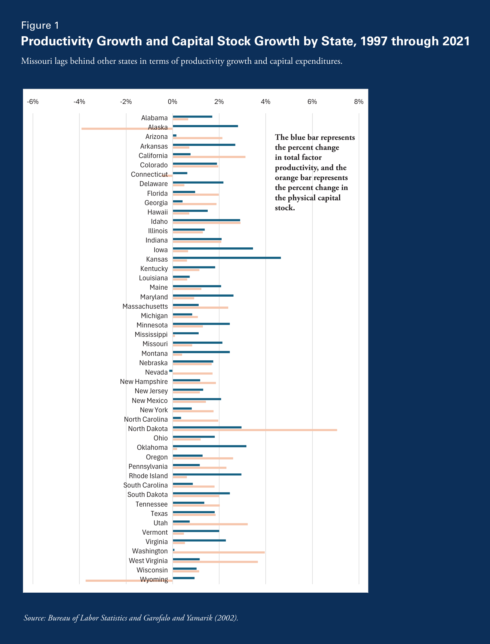
Across states, Missouri is ranked as the 44th fastest-growing state during this period. During the same period, payroll employment increased at a 0.35 percent average annual rate, and the capital stock increased at a 1.45 percent average annual rate. Lastly, TFP increased at a 0.64 percent average annual rate in Missouri between 1997 and 2021. Note that Missouri also ranked as the 44th fastest-growing state in terms of TFP.
Looking across states, we start by calculating how closely correlated the growth rates in these two measures of productivity (labor productivity and TFP) are. For the data covering 2007 to 2021, the estimated correlation coefficient is 0.57. It is comforting to find that there is a positive correlation between labor productivity growth and TFP growth. However, the correlation is sufficiently weak to indicate that by including capital growth, labor productivity is capturing both TFP growth and capital growth. Since labor productivity includes both TFP and capital per worker, the fact that it is not more tightly correlated with TFP growth indicates that it is capturing changes in capital per worker as well.
We also consider the correlation coefficient between TFP growth, employment growth, capital stock growth, and real GDP growth. For the 1997–2021 sample, Table 3 reports the correlation coefficients taken from the growth accounting across states. More specifically, the question is whether movements in real GDP growth, employment growth, capital growth, and TFP growth are correlated across states.
Table 3
Correlation Coefficients from Growth Accounting, 1997–2021
Income growth is driven by the big three; workers, capital expenditures, and productivity.
| Real GDP Growth | Empl. Growth | Capital Growth | TFP Growth | |
|---|---|---|---|---|
| Real GDP Growth | 1 | |||
| Empl. Growth | 0.833 | 1 | ||
| Capital Growth | 0.768 | 0.531 | 1 | |
| TFP Growth | 0.663 | 0.328 | 0.205 | 1 |
Source: Authors’ calculations
Across states, faster real GDP growth is highly correlated with faster employment growth, faster capital growth, and faster TFP growth, meaning that states with stronger economic growth tend to exhibit these characteristics as well.
However, the correlation between employment growth and capital growth and TFP growth, though positive, is much weaker. Overall, the evidence does support the notion that states with faster productivity growth tend to have faster employment growth.
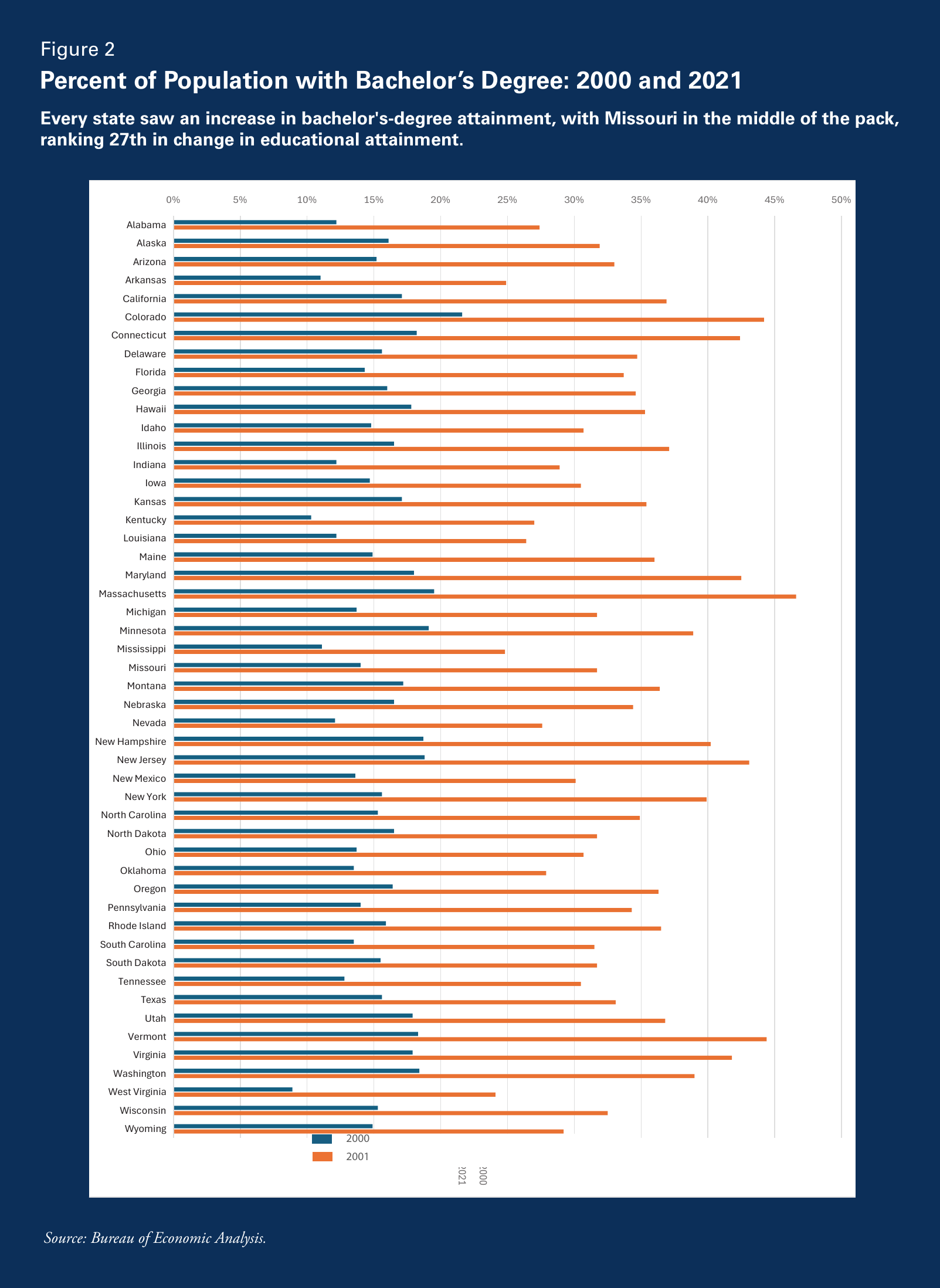
We are interested in how growth is correlated with educational attainment across states. We have the percent of population with bachelor’s degree as the measure of human capital. We have values from the 2000 Census and the 2021 Current Population Survey plotted in Figure 2. A clear observation in the data is the gain in educational attainment in every state over the 21-year period. Thus, there is clear evidence of human capital investment in each state. Massachusetts reports a 27-percentage-point increase in the percent of population with a bachelor’s degree between 2000 and 2021. Missouri reported a nearly 18-percentage-point increase in the percent of population with a bachelor’s degree between 2000 and 2021. Missouri tied for the 27th-largest increase in the change in educational attainment among the states.
The evidence suggests that states with faster productivity growth do, on average, have higher educational attainment levels. The correlation is statistically significant, but the coefficient is small. The results are as follows. Based on the educational attainment level in 2000, real GDP growth is positively correlated with educational attainment and the coefficient equal to 0.39. Alternatively, using the educational attainment level in 2021, the correlation coefficient is 0.24 between real GDP growth and educational attainment. A third correlation is calculated for the change in educational attainment, measured as the difference between educational attainment in 2021 less educational attainment in 2000. The correlation coefficient is 0.1 between real GDP growth and the change in educational attainment.
The evidence suggests that TFP is more closely correlated with educational attainment than real GDP growth is, but only incrementally. With educational attainment measured in 2000, the correlation between TFP growth and educational attainment is 0.51. If we use educational attainment in 2021 as the measure of human capital, the correlation coefficient is 0.34. Lastly, with the change in educational attainment, the correlation coefficient is 0.17 between TFP growth and the changes in educational attainment. The evidence, therefore, indicates that states with higher educational attainment levels are, on average, states that report higher total factor productivity growth. In each case, the correlation is statistically significant.7
Taxes and Growth
In this last section, we present a simple mechanism through which changes in tax rates affect changes in economic growth. The key mechanism is the return to input.
The work by Romer (1986), Lucas (1988), Jones and Manuelli (1990), and Rebelo (1991) sparked a revolution in the way researchers thought about economic growth. Earlier approaches treated technological progress as something that occurred outside the economy. In contrast, this research showed that growth is influenced by the decisions of individuals and firms, particularly their incentives to invest, innovate, and accumulate knowledge. People’s responses to incentives are reflected in the economy as changes in TFP.
There is a common thread across each technological development. Specifically, the key incentive is the return to investing in things that generate faster productivity growth and ultimately, high growth rates. Put more simply, people balance the trade-off between consuming today with the opportunity of greater (expected) consumption in the future. Future consumption gains are achieved by making the economic pie bigger for a given population. And that bigger pie comes from accumulating knowledge and investing in new methods, new technologies, and consequently, productivity gains. The economic process is analogous to sowing and reaping.
As with forward-looking economic decisions, how much to reap and sow depends on the expected return. The expected return is measured in terms of dollars spent today on the investment and the future dollars received—that is, income generated—by the investment. Moreover, it is the after-tax returns that matter to the investor. The equation derived from this problem indicates that the growth rate of income is a function of the expected real, after-tax return on the investment.
Now, we can see clearly how income tax rates affect growth. Growth depends on after-tax returns. And after-tax returns are negatively related to income tax rates. The intuition is straightforward. A higher income tax rate, for example, reduces the after-tax real return on investments. With the decline in the after-tax real return, the incentive to invest declines and correspondingly, the growth rate declines.
In an earlier paper, Castell and Haslag (2010) calculated the effects of state income tax reduction on real GDP growth. Their analysis predicted that real GDP growth rates would increase about 80 basis points given a six-percentage-point decrease in the state income tax. Using an endogenous growth model that incorporates the impact of productivity on economic growth rates, Crader and Haslag (2019) find that state income tax elimination would add a projected 25 to 50 basis points to the average annual economic growth rate.8
In a recent report, the White House Council of Economic Advisers (CEA) looked at the impact that reducing state income tax rates would have on the user cost of physical capital investment. The CEA asked how big the gain to median annual income would be if state income taxes were eliminated. Based on the CEA’s projections, median annual income would rise by nearly $2,900 from ending the state income tax.
The growth model presented above is different in that the projection is a once-and-for-all increase in the growth rate. Compounding would increase the impact of a modest 25-basis-point increase in Missouri’s GDP growth rate such that income would be nearly $1,800 higher in 2035 without the state income tax, and $2,900 if the growth rate increases by 50 basis points. Because these models capture different mechanisms, their wage impacts are additive, so the boost to median annual income could be about $5,800.
Conclusions
Just as Adam Smith used economics to study the determinants of the wealth of nations, the tools of modern economic analysis allow us to study the wealth of states. Despite being part of the same country, some states consistently outpace others in annual economic growth, and with it, wages and incomes. The analysis in this paper reveals that growth differences are no fluke. The single biggest driver of economic growth is labor productivity growth. This insight has major implications for state policy, ranging from tax policy to regulations to education policy. Unfortunately, Missouri has for years demonstrated low productivity growth and economic growth relative to many other states in the country, but proposals to eliminate the income tax could make significant progress in pushing Missouri closer to the front of the pack.
Notes
- State-level capital stock data are available for download at https://cfds.henuecon.education/index.php/data/yes-capital-data. ↩
- See, for example, the discussion by Anderson and Geras (2022) or the discussion in Chapter 11 of Champ, Freeman and Haslag (2022). ↩
- Missouri reported that real GDP increased at 0.92 percent average annual rate between 2007 and 2023. ↩
- The statistical significance means that if one were to suppose that the estimated coefficient is equal to zero, there is less than a one-percent probability that the hypothesis is supported by the data. More formally, one would reject the null hypothesis that there is no relationship between real personal income growth and labor productivity growth across states. ↩
- To be more clear about the distinction between correlation and causation, it is important to put appropriate limits on interpreting these correlations. What we have is evidence suggesting that states with faster employment growth in these six sectors tend to be states with faster income growth. There is also some evidence suggesting that faster employment growth in several sectors indicates a positive relationship between labor productivity growth across states. However, there is no causal link in these simple correlations. To illustrate on the supply side, faster employment growth means increases in workers and their pay; that leads to labor income rising, resulting in faster income growth. Income growth can also arise because of capital deepening; in other words, more investment in physical capital per worker will result in faster income growth. Through greater demand for products, faster employment growth can follow faster income growth. The simple correlation cannot identify which process is driving the results in Table 2. ↩
- Those with calculus backgrounds can do a logarithmic transform of equation 2 and take the derivative with respect to time. ↩
- Compared with the correlation coefficient reported with real GDP growth, the modest increase in the correlation coefficient between TFP and educational attainment suggests that educational attainment is negatively correlated with the sum of employment growth and physical capital growth. In other words, states with higher educational attainment tend to have a lower sum of employment growth and physical capital growth. Such evidence suggests that more educated workers can substitute for the sum of workers and physical capital. More productive workers reduce the sum of workers and capital required. ↩
- Based on a reduction in the average effective income tax rate from 3.5 percent to zero. ↩
References
Anderson, R.B. and M. Geras, 2022. “Correlation Versus Causation.” In: Encyclopedia of Big Data, Laurie A. Schintler and Connie L. McNeely, eds, Cham, Switzerland: Springer Cam.
Casteel, Grant and Joseph H. Haslag, Joseph H. 2011. “Income Taxes vs. Sales Taxes: A Welfare Comparison,” Show-Me Institute Essay. December 2010.
Chamo, Bruce, Scott Freeman and Joseph H. Haslag, 2022. Modeling Monetary Economies, Cambridge, UK: Cambridge University Press.
Crader, G. Dean and Joseph H. Haslag, 2019. “Computing State Average Marginal Income Tax Rates: An Application to Missouri,” Growth and Change, 50(1):424–45.
Garofalo, Gasper A. and Steven Yamarik, 2002. “Regional Convergence: Evidence from a new State-by-State Capital Stock Series,” The Review of Economics and Statistics, 84(2):316–23.
Jones, Larry E. and Rodolfo Manuelli, 1990. “A Convex Model of Equilibrium Growth: Theory and Policy Implications,” Journal of Political Economy, 98(5, Part1):1008–38.
Lucas, Robert E., Jr., 1988. “On the Mechanics of Economic Development,” Journal of Monetary Economics, 22:3–42.
Rebelo, Sergio, 1991. “Long-run Policy Analysis and Long-run Growth,” Journal of Political Economy, 99(3):500–21.
Romer, Paul M. 1986. “Increasing Returns and Long-run Growth,” Journal of Political Economy, 94:1002–37.
White House Council of Economic Advisers, 2026. “The Economic Impact of State Income Tax Elimination.” https://www.whitehouse.gov/wp-content/uploads/2025/03/The-Economic-Impact-of-State-Income-Tax-Elimination.pdf.
Yamarik, Steven and Makram El-Shagi, 2019. “State-level Capital and Investment: Refinements and Updates,” Growth and Change, 50(4):1411–22.